Analysing mtDNA cell lines in bulk RNA seq data
Source:vignettes/cell_competition_bulk_data_mt_example_notebook.Rmd
cell_competition_bulk_data_mt_example_notebook.Rmd
library(MitoHEAR)In this notebook it is shown the heteroplasmy analysis performed on bulk RNA seq mouse data from Lima et al, 2021. There are in total 8 samples that belong to the cell line BG (95%) and 8 samples that belong to the cell line HB (24%). The two cell lines are built in order to have a different mitochondrial DNA from each other and from the reference genome in some bases. The cell lines BG and HB are respectively classified as Loser and Winner.
Get counts for the four alleles in each base-sample pair
The first step of the library MitoHEAR is to generate a raw counts allele matrix with cells as rows and the four alleles for each base in the fasta file on the columns. This task is achieved with the function get_raw_counts_allele. As input we need to provide the sorted bam files (one for each cell, with full path), the fasta file of the genomic region of interest and the cell names. The matrices meta_data_ana_final_big and meta_data_ana_final_small contain meta data information about the cells (i.e. cell names, condition).
load(system.file("extdata", "meta_data_ana_final_big.Rda", package = "MitoHEAR"))
load(system.file("extdata", "meta_data_ana_final_small.Rda", package = "MitoHEAR"))
cell_names <- as.vector(meta_data_ana_final_big$name_cell)
cell_names_bulk <- cell_names
We don’t execute the function get_raw_counts_allele here and we directly load his output. A command line implementation of the function get_raw_counts_allele is also available (see github README file for info).
load(system.file("extdata", "output_SNP_ana_mt.Rda", package = "MitoHEAR"))The output of get_raw_counts_allele is a list with three elements (see ?get_raw_counts_allele for more info). The first element is the matrix of counts (n_rows = number of cells, n_cols= 4*number of bases) of the four alleles in each base. The row names are equal to cell_names.
matrix_allele_counts <- output_SNP_ana_mt[[1]]
name_position_allele <- output_SNP_ana_mt[[2]]
name_position <- output_SNP_ana_mt[[3]]
row.names(meta_data_ana_final_big) <- meta_data_ana_final_big$name_cell
meta_data_ana_final_big <- meta_data_ana_final_big[row.names(matrix_allele_counts),]
delete_duplicate <- meta_data_ana_final_big$name_cell[seq(1,48,3)]
meta_data_ana_final_big_filter <- meta_data_ana_final_big[delete_duplicate,]
bulk_sample <- meta_data_ana_final_big_filter$name_cell_original

matrix_allele_counts <- matrix_allele_counts[delete_duplicate,]
row.names(matrix_allele_counts) <- bulk_sample


row.names(meta_data_ana_final_small) <- meta_data_ana_final_small$name_fastq
The next step is to obtain a matrix with allele frequencies and a matrix with heteroplasmy values for each pair of cell-base. This is obtained with the function get_heteroplasmy. This function performs a two step filtering procedure, the first on the cells and the second on the bases. The aim is to keep only the cells that have more than number_reads counts in more than number_positions bases and to keep only the bases that are covered by more than number_reads counts in all the cells (filtering=1) or in at least 50% of cells in each cluster (filtering=2).
bulk_data_competition <- get_heteroplasmy(matrix_allele_counts[bulk_sample,],name_position_allele,name_position,50,2000,filtering = 1)Among the output of get_heteroplasmy there are the matrix with heteroplasmy values and the matrix with allele frequencies, for all the cells and bases that pass the two step filtering procedure. The heteroplasmy is computed as 1-max(f), where f are the frequencies of the four alleles for every cell-base pair. For more info about the output see ?get_heteroplasmy.
sum_matrix <- bulk_data_competition[[1]]
sum_matrix_qc <- bulk_data_competition[[2]]
heteroplasmy_matrix_bulk <- bulk_data_competition[[3]]
allele_matrix_bulk <- bulk_data_competition[[4]]
cluster_bulk <- as.character(meta_data_ana_final_small[row.names(heteroplasmy_matrix_bulk),]$status)
condition_bulk <- as.character(meta_data_ana_final_small[row.names(heteroplasmy_matrix_bulk),]$condition)
index_bulk <- bulk_data_competition[[5]]
name_position_allele_qc <- name_position_allele[name_position%in%colnames(sum_matrix_qc)]
name_position_qc <- name_position[name_position%in%colnames(sum_matrix_qc)]
It is possible to perform an additional filtering step on the bases keeping only the ones with an heteroplasmy value above min_heteroplasmy in more than min_cells.
relevant_bases <- filter_bases(heteroplasmy_matrix_bulk,0.01,8)Identification of most different bases according to heteroplasmy between clusters
For detecting the difference in heteroplasmy values between two group of cells (i.e. two clusters), an unpaired two-samples Wilcoxon test is performed. In this case we run the test between the groups Winner and Loser. As output, for each bases, there is the adjusted p value (FDR).
p_value_wilcox_test <- get_wilcox_test(heteroplasmy_matrix_bulk[,relevant_bases],cluster_bulk,"Loser","Winner" )We sort the bases according to the adjusted p value in order to identify the bases where the heteroplasmy is most different between the two groups.
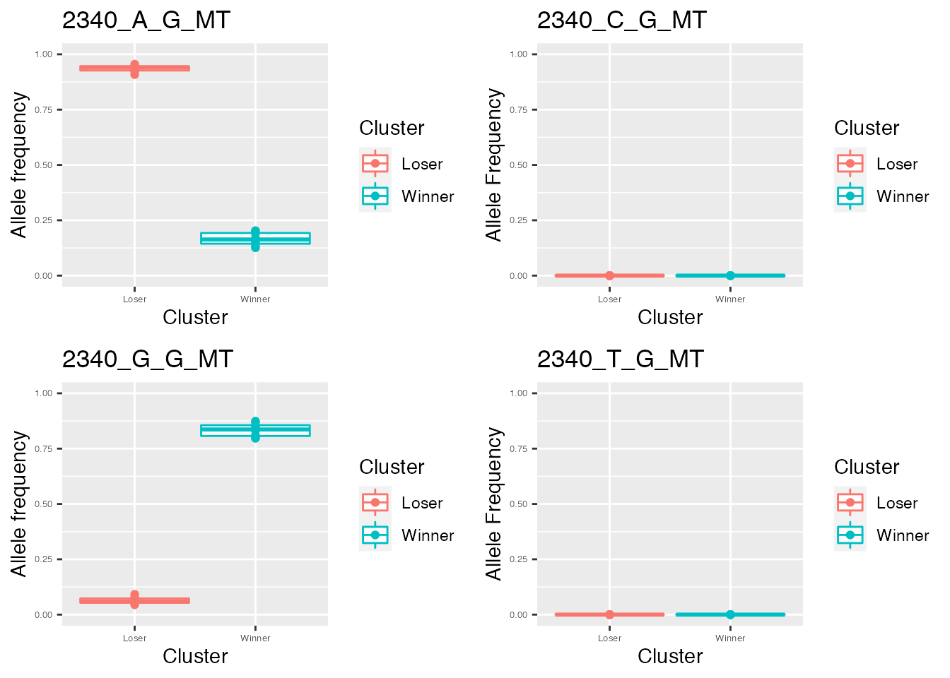
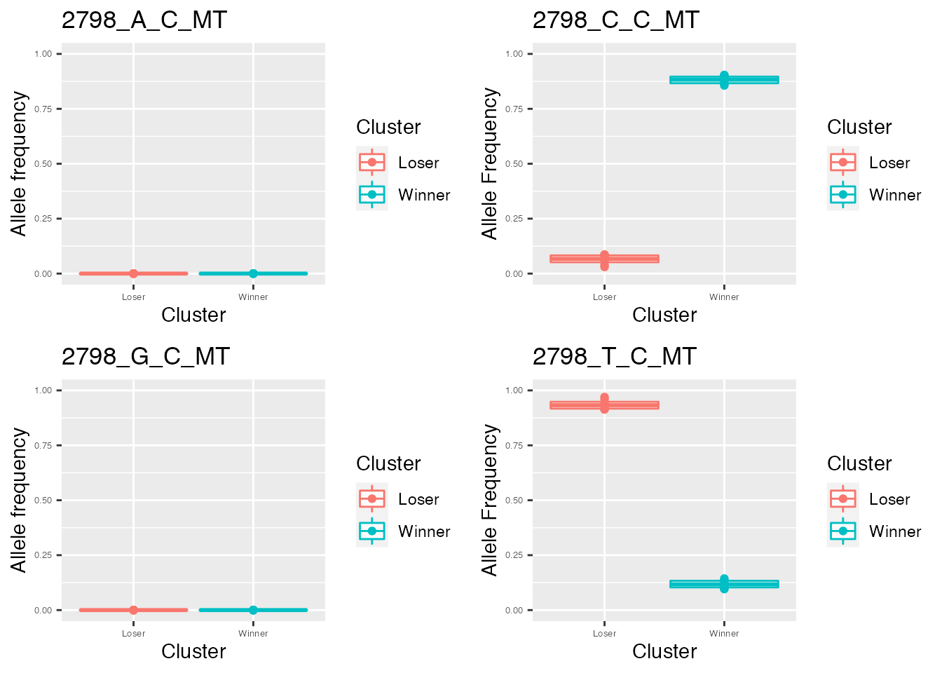
p_value_wilcox_test_sort <- sort(p_value_wilcox_test,decreasing = F)The heteroplasmy and the corresponding allele frequencies for the most relevant bases (according to Wilcoxon test) are shown. The difference in heteroplasmy values is sharp, as expected since the two cell lineages (Winner and Loser) have a different mitochondrial DNA by construction.
q <- list()
for ( i in 1:length(p_value_wilcox_test_sort[1:2])) {
p <- plot_heteroplasmy(names(p_value_wilcox_test_sort)[i],heteroplasmy_matrix_bulk,cluster_bulk,index_bulk)+ggplot2::ggtitle(paste(names(p_value_wilcox_test_sort)[i],round(p_value_wilcox_test_sort[i],4),sep = "-"))
q <- list(q,p)
}
q
#> [[1]]
#> [[1]][[1]]
#> list()
#>
#> [[1]][[2]]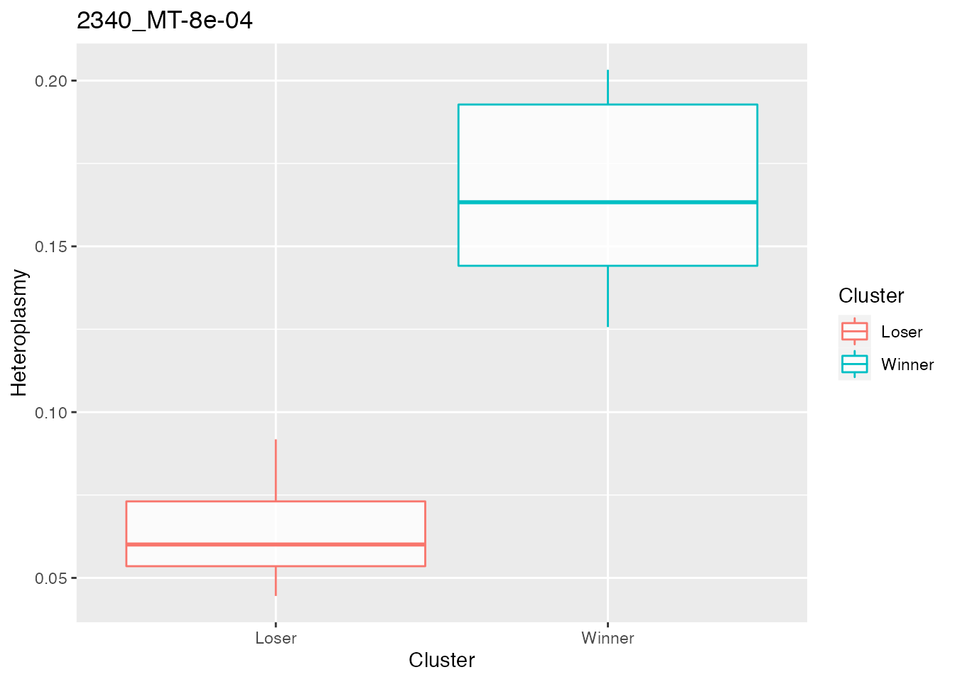
#>
#>
#> [[2]]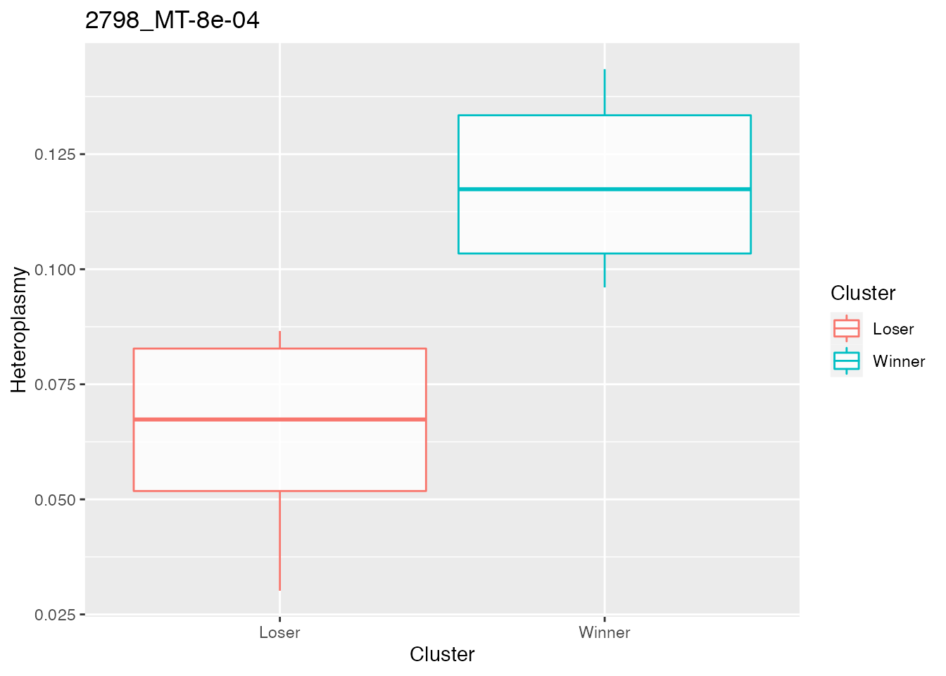
q <- list()
for ( i in names(p_value_wilcox_test_sort)[1:2]) {
p <- plot_allele_frequency(i,heteroplasmy_matrix_bulk,allele_matrix_bulk,cluster_bulk,name_position_qc,name_position_allele_qc,5,index_bulk)
q <- list(q,p)
}
q
#> [[1]]
#> [[1]][[1]]
#> list()
#>
#> [[1]][[2]]
#> TableGrob (2 x 2) "arrange": 4 grobs
#>   z     cells    name           grob
#> 1 1 (1-1,1-1) arrange gtable[layout]
#> 2 2 (1-1,2-2) arrange gtable[layout]
#> 3 3 (2-2,1-1) arrange gtable[layout]
#> 4 4 (2-2,2-2) arrange gtable[layout]
#>
#>
#> [[2]]
#> TableGrob (2 x 2) "arrange": 4 grobs
#>   z     cells    name           grob
#> 1 1 (1-1,1-1) arrange gtable[layout]
#> 2 2 (1-1,2-2) arrange gtable[layout]
#> 3 3 (2-2,1-1) arrange gtable[layout]
#> 4 4 (2-2,2-2) arrange gtable[layout]
We can check if there is a batch effect in the most relevant positions (i.e. the heteroplasmy levels are constantly higher only in a specific batch). For the top 2 positions defined with the GAM fit there is not a batch effect, since the difference in heteroplasmy levels are driven by group (Winner and Loser) and not by batch (co cultured-CO or separate culture-Sep).
utile <- meta_data_ana_final_small[row.names(heteroplasmy_matrix_bulk),]
batch <- rep(0,length(utile$condition))
batch[utile$status == "Loser"&utile$condition == "CO"] <- "Loser-CO"
batch[utile$status == "Loser"&utile$condition == "Sep"] <- "Loser-Sep"
batch[utile$status == "Winner"&utile$condition == "CO"] <- "Winner-CO"
batch[utile$status == "Winner"&utile$condition == "Sep"] <- "Winner-Sep"


cluster <- utile$status

q <- list()
for ( i in names(p_value_wilcox_test_sort)[1:2]) {
p <- plot_batch(i, heteroplasmy_matrix_bulk, batch, cluster, 6, index_bulk)
q <- list(q, p)
}
q
#> [[1]]
#> [[1]][[1]]
#> list()
#>
#> [[1]][[2]]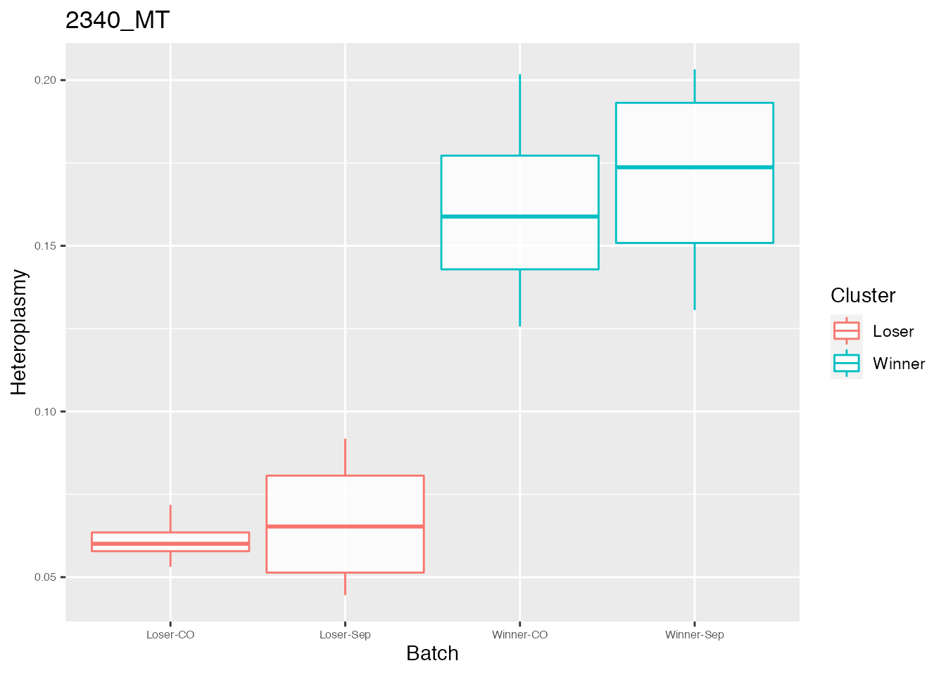
#>
#>
#> [[2]]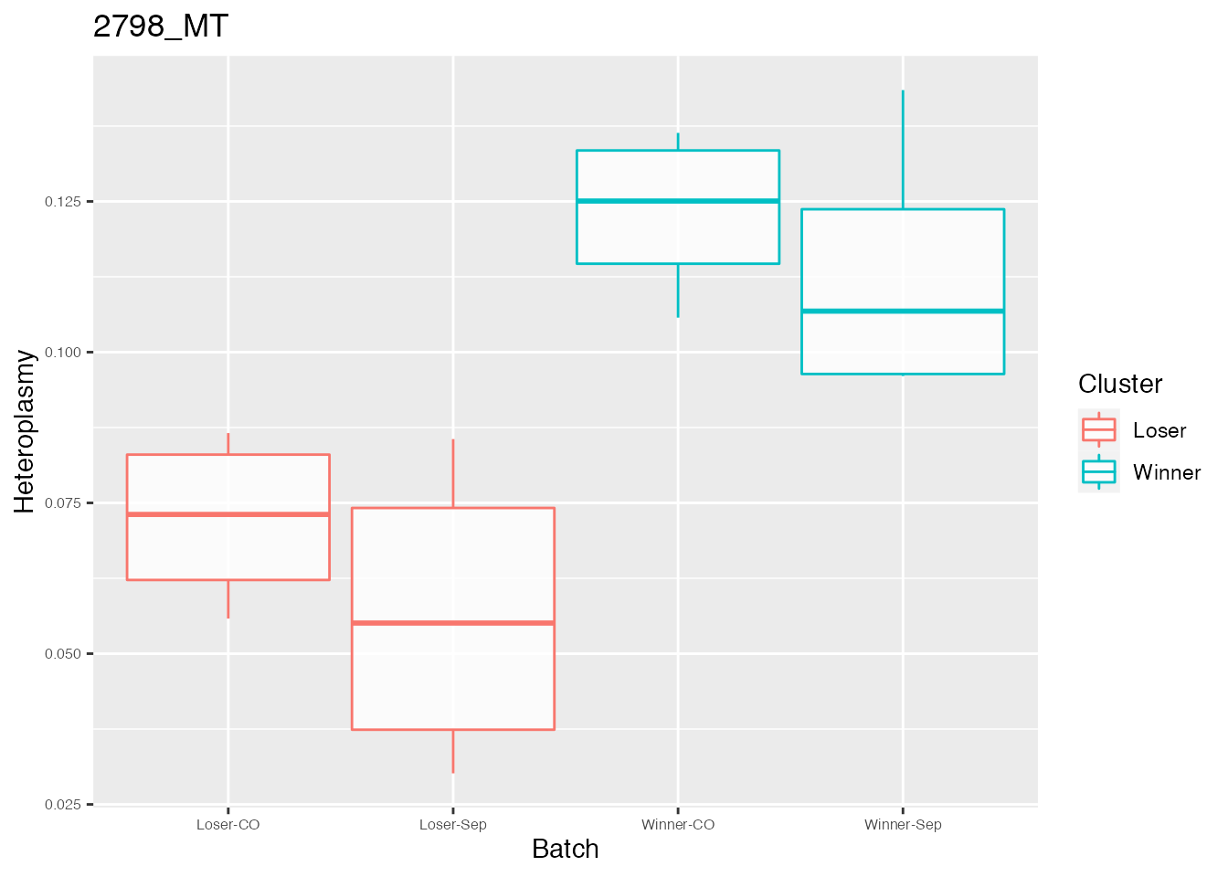
Unsupervised cluster analysis among cells based on allele frequency values
MitoHEAR offers the possibility to perform an unsupervised hierarchical clustering on the cells based on a distance matrix with the function clustering_dist_ang. Given a base, the distance between two cells is the angular distance of the allele frequencies. Given a base, the variance of the distance values between two cells is also computed. Top bases with highest variance are selected for down stream analysis. We can represent the difference between two cells as a vector whose coordinates are the angular distances of the top bases. The total distance between two cell is the euclidean norm of the vector of difference between the two cells. The output of clustering_dist_ang is a list. The first element is a data frame which contains the old classification (partition available before the cluster analysis based on allele frequencies) and the new classification (partition provided by the cluster analysis based on allele frequencies ). The second element is the distance matrix, on which the hierarchical clustering is done. The third element is a vector with the top bases according to variance.
It is also possible to run clustering_dist_ang in a supervised approach. In this case the bases used for hierarchical clustering are not selected according to variance, but are directly provided with the parameter relevant_bases. The heatmap of the distance matrix with cells sorted according to the new classification is shown below. The cluster analysis based on allele frequencies information can be a powerful way to perform a lineage tracing analysis, by grouping together cells which are from the same embryo. See ?clustering_dist_ang for more info.
result_clustering_sc <- clustering_angular_distance(heteroplasmy_matrix_bulk, allele_matrix_bulk, cluster_bulk, length(colnames(heteroplasmy_matrix_bulk)), deepSplit_param = 1, minClusterSize_param = 8, 0.2, min_value = 0.001, index = index_bulk, relevant_bases = NULL)
#>  ..cutHeight not given, setting it to 11.3  ===>  99% of the (truncated) height range in dendro.
#>  ..done.


old_new_classification <- result_clustering_sc[[1]]
dist_matrix_sc <- result_clustering_sc[[2]]
top_dist <- result_clustering_sc[[3]]
common_idx <- result_clustering_sc[[4]]

old_classification <- as.vector(old_new_classification[, 1])
new_classification <- as.vector(old_new_classification[, 2])

plot_distance_matrix(dist_matrix_sc, old_classification)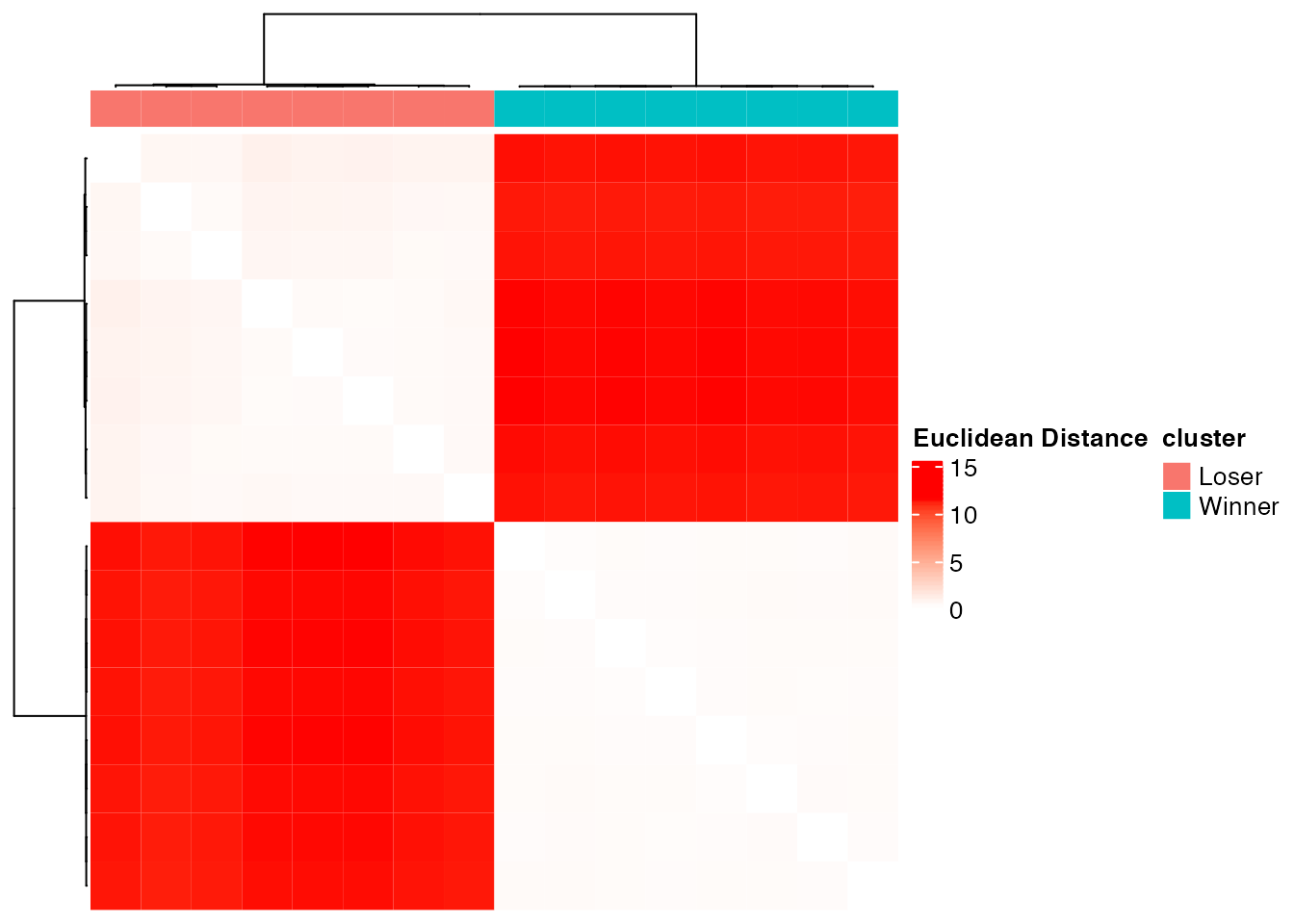
Below we plot the top 2 bases selected for the unsupervised cluster analysis
q <- list()
for ( i in 1:length(top_dist[1:2])) {
p <- plot_heteroplasmy(top_dist[i], heteroplasmy_matrix_bulk, cluster_bulk, index_bulk)
q <- list(q, p)
}
q
#> [[1]]
#> [[1]][[1]]
#> list()
#>
#> [[1]][[2]]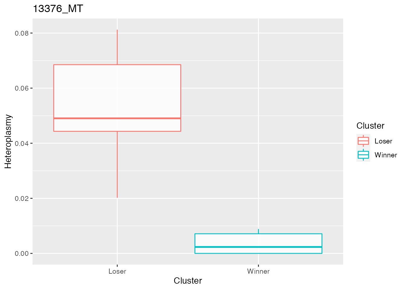
#>
#>
#> [[2]]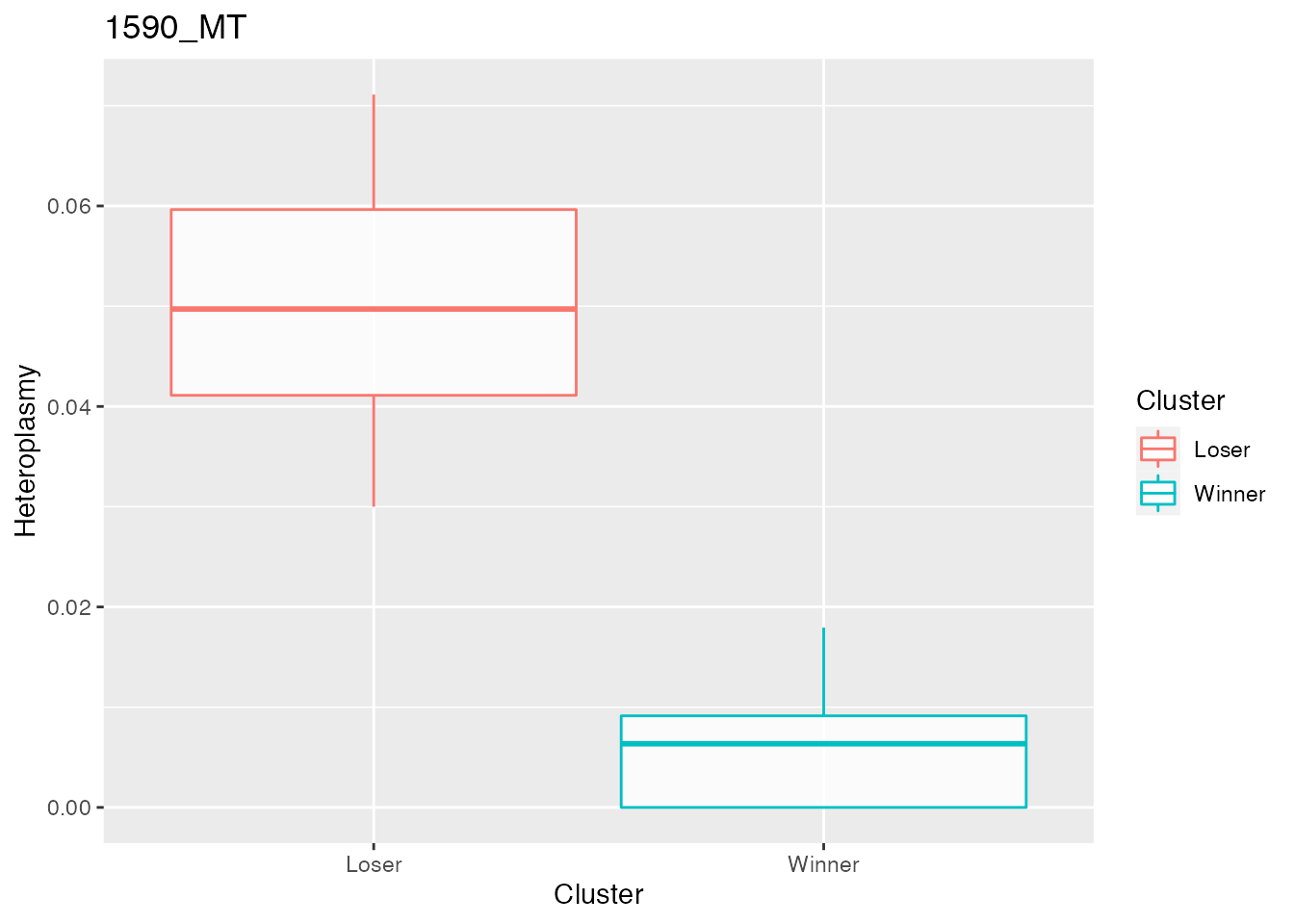
Comparison between the ground truth and the new partition obtained with unsupervised cluster analysis
plot_heatmap(new_classification, old_classification, (dist_matrix_sc), cluster_columns = F, cluster_rows = F, "Euclidean distance")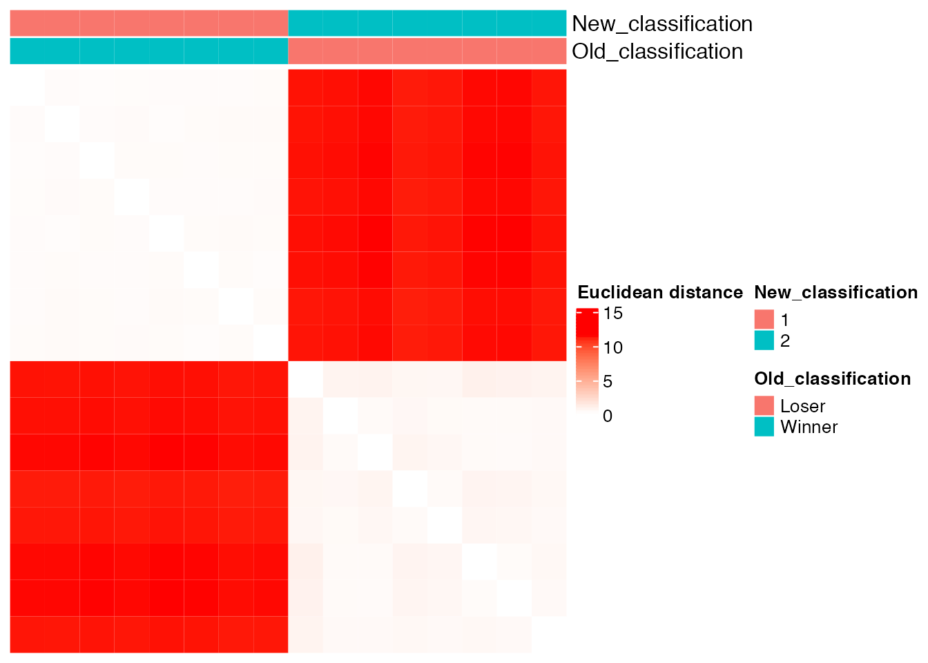
The new classification coincides with the old classification. This means that we can perfectly distinguish between the two cell lines only by looking at the heteroplasmy values of the mitochondrial bases. This result was expected since the samples derived from two cell lines, whose mitochondrial DNA is built to be different between each other.
utils::sessionInfo()
#> R version 4.0.2 (2020-06-22)
#> Platform: x86_64-apple-darwin17.0 (64-bit)
#> Running under: macOS Mojave 10.14.6
#>
#> Matrix products: default
#> BLAS:   /Library/Frameworks/R.framework/Versions/4.0/Resources/lib/libRblas.dylib
#> LAPACK: /Library/Frameworks/R.framework/Versions/4.0/Resources/lib/libRlapack.dylib
#>
#> locale:
#> [1] en_US.UTF-8/en_US.UTF-8/en_US.UTF-8/C/en_US.UTF-8/en_US.UTF-8
#>
#> attached base packages:
#> [1] stats     graphics  grDevices utils     datasets  methods   base
#>
#> other attached packages:
#> [1] MitoHEAR_0.1.0
#>
#> loaded via a namespace (and not attached):
#>  [1] Rcpp_1.0.7            circlize_0.4.13       png_0.1-7
#>  [4] assertthat_0.2.1      rprojroot_2.0.2       digest_0.6.29
#>  [7] utf8_1.2.2            R6_2.5.1              dynamicTreeCut_1.63-1
#> [10] stats4_4.0.2          evaluate_0.14         ggplot2_3.3.5
#> [13] highr_0.9             pillar_1.6.4          GlobalOptions_0.1.2
#> [16] rlang_0.4.12          jquerylib_0.1.4       magick_2.7.3
#> [19] S4Vectors_0.28.1      GetoptLong_1.0.5      rmarkdown_2.11
#> [22] pkgdown_2.0.2         textshaping_0.3.6     desc_1.2.0
#> [25] labeling_0.4.2        stringr_1.4.0         munsell_0.5.0
#> [28] compiler_4.0.2        xfun_0.29             pkgconfig_2.0.3
#> [31] systemfonts_1.0.4     BiocGenerics_0.36.1   shape_1.4.6
#> [34] htmltools_0.5.2       tidyselect_1.1.1      tibble_3.1.6
#> [37] gridExtra_2.3         IRanges_2.24.1        matrixStats_0.61.0
#> [40] fansi_0.5.0           crayon_1.4.2          dplyr_1.0.7
#> [43] grid_4.0.2            jsonlite_1.7.2        gtable_0.3.0
#> [46] lifecycle_1.0.1       DBI_1.1.2             magrittr_2.0.1
#> [49] scales_1.1.1          stringi_1.7.6         cachem_1.0.6
#> [52] farver_2.1.0          fs_1.5.2              bslib_0.3.1
#> [55] ellipsis_0.3.2        ragg_1.2.2            generics_0.1.1
#> [58] vctrs_0.3.8           rdist_0.0.5           RColorBrewer_1.1-2
#> [61] rjson_0.2.20          tools_4.0.2           Cairo_1.5-12.2
#> [64] glue_1.6.0            purrr_0.3.4           parallel_4.0.2
#> [67] fastmap_1.1.0         yaml_2.2.1            clue_0.3-60
#> [70] colorspace_2.0-2      cluster_2.1.0         ComplexHeatmap_2.6.2
#> [73] memoise_2.0.1         knitr_1.37            sass_0.4.0